Transformer learning notes: from the overall architecture to multi-head attention

Summary

Transformer study notes ordered whole-first and then part-by-part: the data flow through the encoder and the decoder; the three questions to answer before learning large models (neural networks, attention, what PyTorch is made of); what Token, the word embedding matrix, and positional encoding each solve; the meaning of Q, K, and V, why the Q·K dot product stands for relevance, and why the dot product is divided by the square root of the dimension before softmax; the difference between self-attention and cross-attention, and why cross-attention needs no mask; training predicts several tokens in parallel while inference generates one token at a time, which is why a causal mask is needed to prevent peeking, implemented by setting later positions to negative infinity so that softmax turns them into 0; the definitions of the feed-forward network, multi-head attention, and layer normalization, including how layer norm and batch norm differ in which dimension they normalize over.

These notes are what I wrote down while learning the Transformer; they were first posted on CSDN. Now that they have moved back to my own site, I have reworked the order and the data flow along the way — the conclusions are unchanged, the explanation just flows a little better.

It is not really a tutorial, more a record of studying: look at the whole first, then take the parts apart one by one.

The big picture first: how the data flows

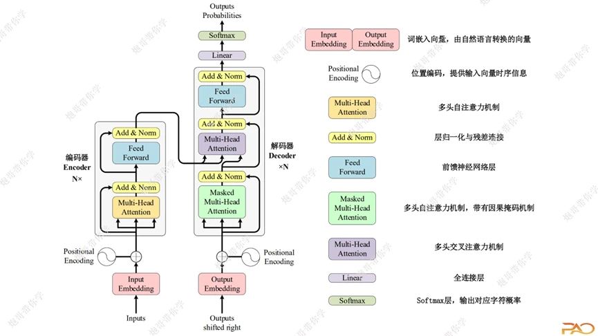
The input first passes through the word embedding matrix, where it is fused with the positional encoding, then enters multi-head attention (Q, K, V), then goes through layer norm and a residual connection, into the feed-forward network, and once more through layer norm and a residual connection. Up to this point we have the input plus the encoder — and the encoder can be stacked N layers deep with that same structure.

On the decoder side, the input starts from <start>, again goes through word embedding and positional encoding first, and then passes through, in order:

causal mask attention → layer norm + residual → cross-attention → layer norm + residual
                      → feed-forward network → layer norm + residual → linear layer → softmax → output

So the whole architecture is nothing more than these few modules, and we can just understand them one by one.

The overall Transformer architecture: the encoder on the left, the decoder on the right, with layer norm and a residual connection after every sublayer

Getting to know large models

We have all used plenty of large models by now, so you will have noticed that after you ask a question, the answer does not come out all at once — it pops out one word at a time, like a word-chain game. Once you have learned the fundamentals of large models and then look back at this process, your understanding of AI becomes much more concrete.

In learning large models and learning about agents, I set myself three questions to answer first.

1. What is a neural network? The most basic answer is that it is the foundation of learning: x -> f(x) -> y.

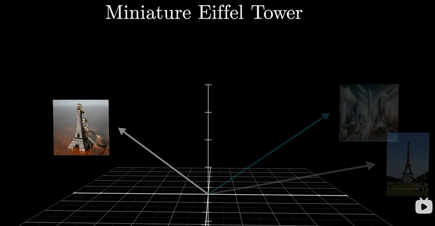
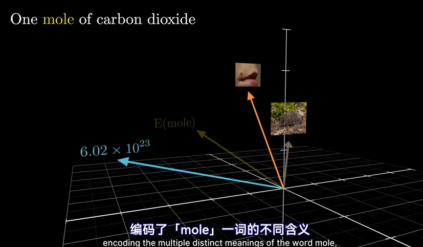
2. What is attention? For your input, I need to allocate different amounts of attention (that is, weight parameters) so that the output moves toward what you want. Looked at spatially: a word (token) has many vector directions, and attention is what turns that word into the vector direction that fits the current meaning.

A sketch of word-vector space: semantic relationships are encoded as directions

3. What is PyTorch made of? Remembering these few parts is enough: Tensor, Parameter (the optimizable parameters, that is, the initialized parameters), Model, Autograd (computing gradients), Optimizer (optimizing the parameters).

Now we can get into the Transformer.

Model components

1. Token

First we need to split a sentence into many words, and such a word is called a token. Take I love you — that is 3 tokens; for now just think of a token as a word.

A computer does not know these words, so they still have to be turned into a language it can recognize — vectors. Each token contains many numbers, and those numbers are hard for us to read directly, but roughly they can represent complex information such as a word’s meaning, part of speech, and position. The same word has different vectors in different sentences.

The same word points in different vector directions in different contexts: mole points along different semantic directions under its two meanings

2. The word embedding matrix

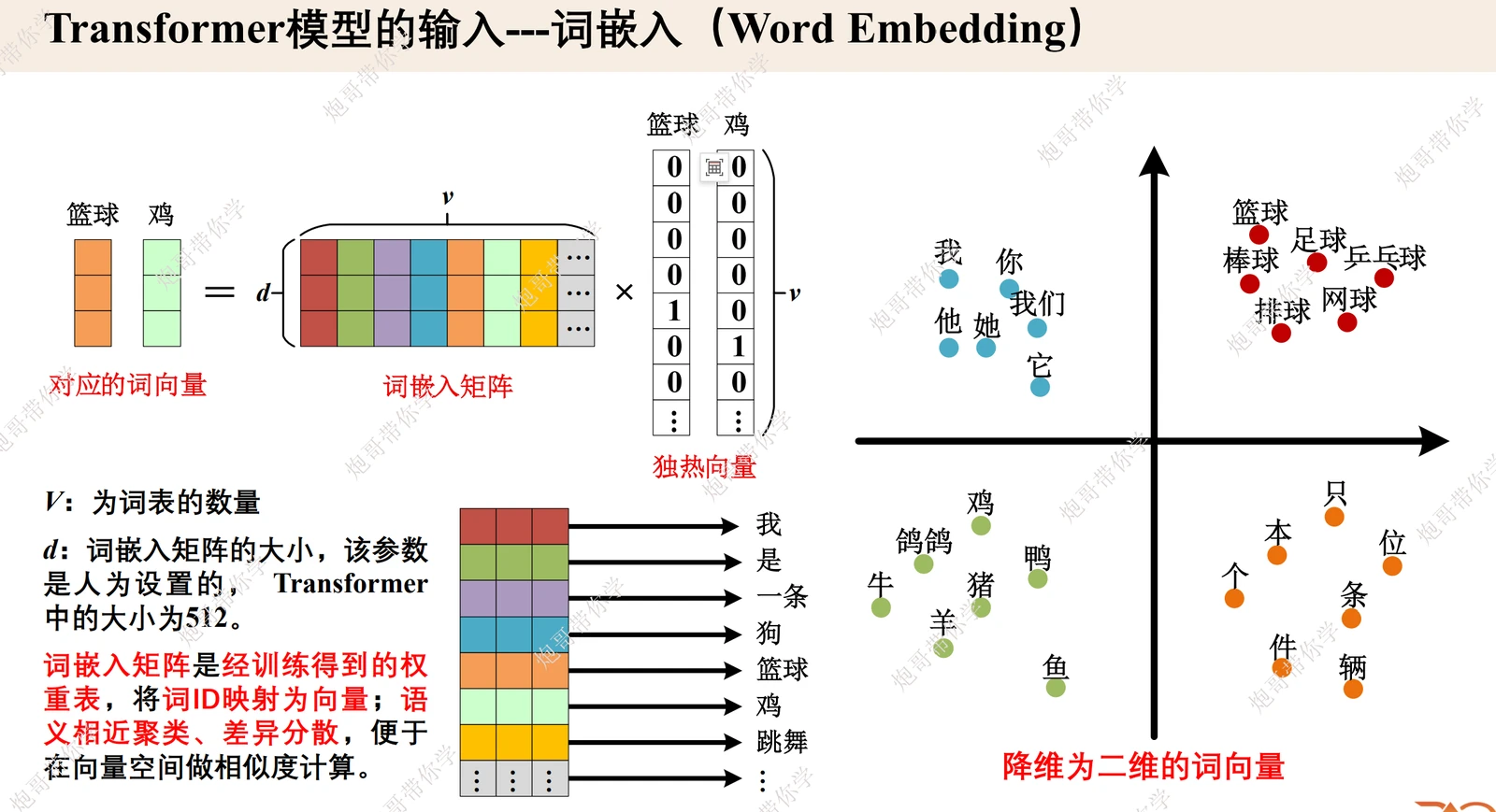
The first approach to handling a token was one-hot encoding (0/1). Take the Chinese sentence 我是一只狗 (“I am a dog”):

我  -> [1, 0, 0, 0, 0, …]
是  -> [0, 1, 0, 0, 0, …]
一  -> [0, 0, 1, 0, 0, …]

The problem is obvious: the dimensionality is huge, and only one position in each vector is 1. So word embeddings come in: through the word embedding matrix (a weight table learned during training), words that are close in meaning cluster together and words that differ greatly spread apart, and dimensionality is reduced at the same time — separating natural language by numbers.

The word vector dimension d is typically 512; it holds the basic semantic information of the token and is a weight table that can be tuned during model training.
V is the vocabulary size, that is, the number of tokens.
The word embedding matrix is d × V; a single token’s one-hot vector is V × 1, and multiplying them gives d × 1. The tokens of a whole sentence combined give V × d.

A diagram of one-hot encoding, the word embedding matrix, and word vectors reduced to two dimensions

3. Positional encoding

At this point the data has in fact already been processed, so why process it a second time? Because what we are dealing with is not data like tables or images but information that carries order and semantic logic. Take 狗咬人 and 人咬狗 (“dog bites man” and “man bites dog”): the words sit in different positions and the meaning is completely different, so we need a piece of information that measures this property.

Positional encoding in the Transformer is a formula built on trigonometric functions; its parameters are the embedding dimension d and the position pos of the current token in the sequence, and the result is added element-wise to the word embeddings.

4. Attention: Q, K, V

At the outset, a token contains only its own vector, but once it enters the Transformer, attention moves that vector to the semantic position that fits the context.

When we predict the next token, the basis is the embedding vector of the previous token; because it already contains the semantics of the context, its parameter count is far larger than that of a single token on its own.

Next come the three most important parameters: Q, K, V.

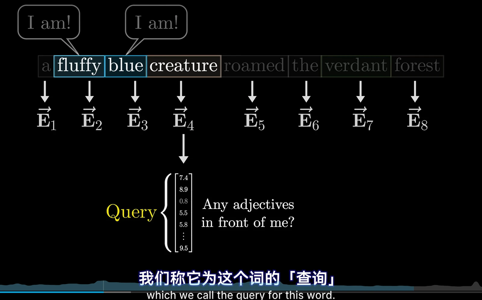
Q (Query): in an English sentence, for instance, a noun asks whether there is an adjective in front of it, and that question is encoded into another vector, the query. In effect, every word queries its own context for information. Q = Wq · E, where Wq is a parameter the model learns; the dimension of Q is far smaller than the dimension of E, which amounts to going from high dimensions down to low ones.

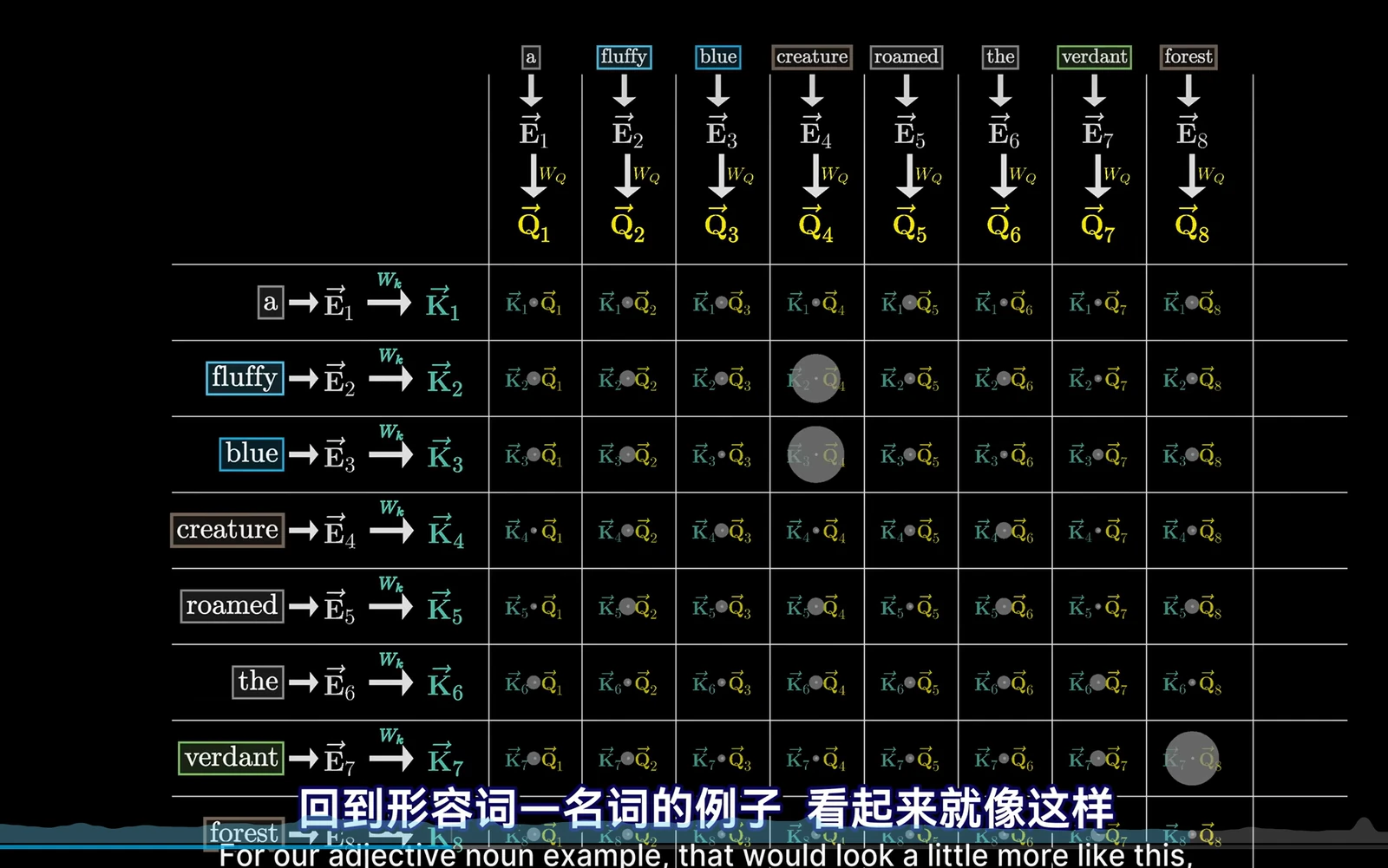
Query illustrated: every word puts a question to its context — is there an adjective in front of me

K (Key): if there really is an adjective in front, then the adjective’s answer becomes the key. Wk is also a learnable parameter, K = Wk · E. So when the noun’s query for an adjective really exists, the relevance is high: the dot product of Q and K is large, and the query and the answer line up.

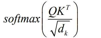
The attention matrix produced by the dot product of Q and K: the relevance score between every two tokens in the sentence

To turn that into probabilities we then pass it through softmax; for numerical stability we first divide by the square root of the dimension.

softmax(QKᵀ / √d_k): after the dot product, divide by the square root of the dimension and then take the softmax to get probabilities

V (Value): the vector you need to add in if you want to change the meaning of a particular word.

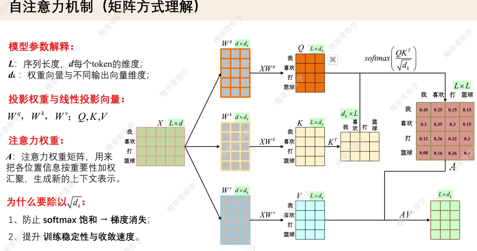
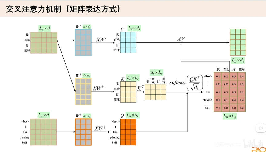
Self-attention in matrix form: X multiplied by Wq, Wk, and Wv gives Q, K, and V

I may not have explained this very well, so I would suggest reading up on it elsewhere as well. What I described above is self-attention; in machine translation there is also cross-attention: words in one language query and answer words in another language, and no mask is used here (more on that later), because there is no “peeking” problem.

Cross-attention in matrix form: Q comes from the decoder, K and V come from the encoder

5. Training and inference

Take a translation task as an example: the input is 我是一条狗 and the labels are I am a dog.

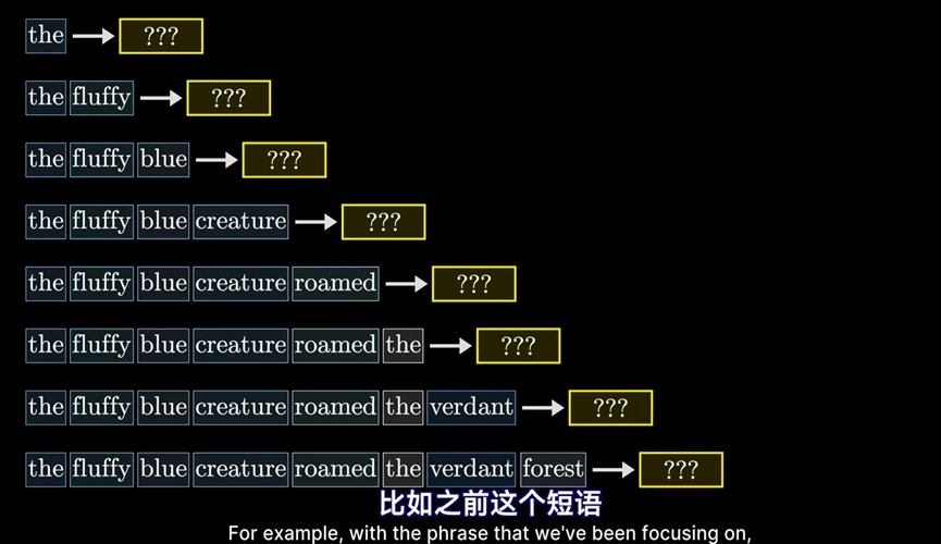
Inference first: the Chinese input goes through the encoder and yields the encoded information; the decoder starts from <start>, combines the neural network’s computation with that encoded information, and produces the highest-probability English word I; then from <start> I it produces am; then from <start> I am it produces a… and so on until the <end> terminator.

So it takes each output together with the previous outputs as input and infers the next output from them.

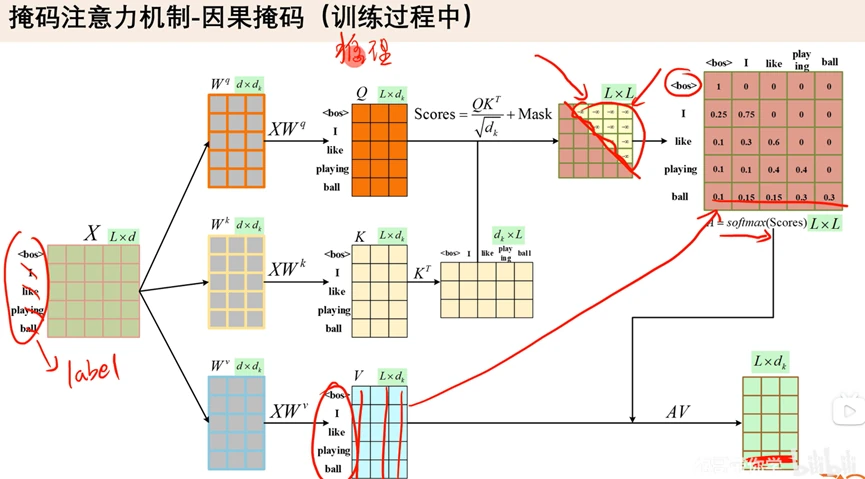
Training is a little different. First, the model makes full use of the data: it predicts several tokens at once, so one sample trains many times over, and the loss is computed in parallel, which speeds things up enormously.

At the same time, we need the model to train in the right direction. Back to the translation task: if the model translates the very first step wrongly, everything after it only goes more wrong. So we tell the model the “correct answer”, making sure it learns under the right conditions. And that is where the problem shows up — the answer has been given to the model, so it can simply read along; what is left to train then? So we introduce a mask into attention, to stop the model from “peeking” and to stop later words from influencing the prediction of earlier ones.

During training several positions are predicted at once, and each position can only see the words before it

6. The causal mask attention mechanism

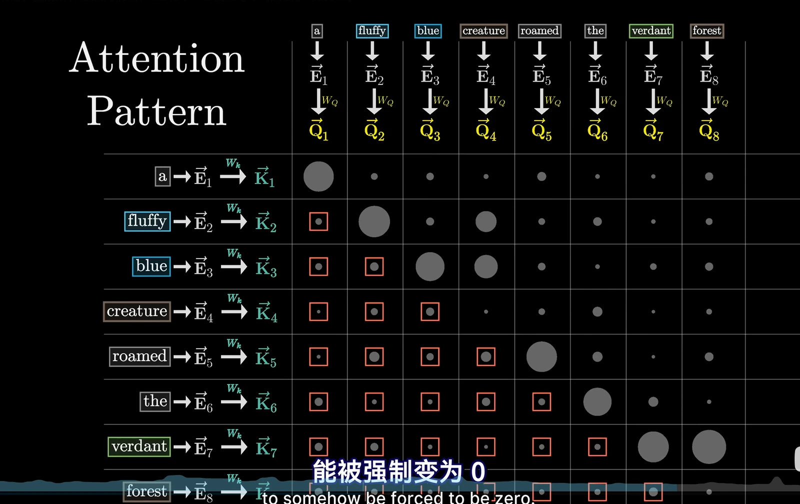
We want this “query” not to be influenced by later words; and since probabilities are what come out in the end, the method is to set the later positions to negative infinity first, which softmax then turns into 0.

The causal mask in matrix form: the masked upper-triangular region is set to negative infinity before softmax

The attention matrix after masking: the upper-triangular region is forced to 0

7. The feed-forward network

A kind of network structure: no recurrence, one-directional flow, multiple layers, mostly fully connected layers. (An RNN is not one; AlexNet is.) This part is relatively simple.

8. Multi-head attention

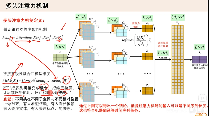
For a set of tokens, several independent attention computations are run on each token. Different attention weights W focus on different angles — the meaning within the sentence, punctuation, syntax, and so on.

Multi-head attention: several independent sets of Wq, Wk, and Wv computed in parallel, then concatenated

9. Layer normalization

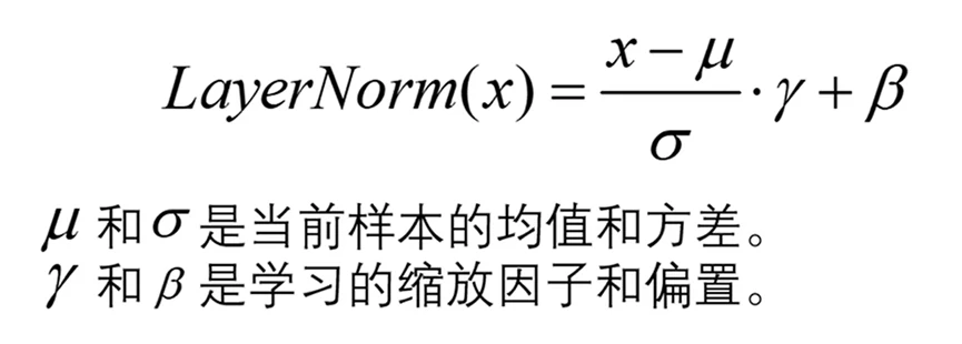
Layer normalization: for one sample, normalize its outputs across all neurons together (y1, y2, y3, y4, …).

Batch normalization (the kind ResNet uses): within the same layer, normalize the outputs of different samples at the same neuron (y1, y1, y1, y1, …).

Normalization	What it normalizes over	Typical use
Layer normalization LayerNorm	The outputs of one sample across all neuron dimensions	After every sublayer in the Transformer
Batch normalization BatchNorm	The outputs at the same neuron across different samples in a batch	Convolutional networks such as ResNet

The LayerNorm formula: subtract the current sample's mean, divide by the standard deviation, then multiply by a scale factor and add a bias

In closing

I am a learner too — at the time I followed the courses by Paoge and 3BB on Bilibili. This article is my own understanding of the Transformer, written only to record my learning process and output; there may be one-sided or wrong points in it, and I warmly welcome corrections so that we can learn together.

The architecture diagrams, formula figures, and matrix screenshots in this article come from the course slides; the word-vector-space illustration comes from Paoge’s channel and 3Blue1Brown’s attention series.